Introduction
Ever since Transformer was introduced in 2017, there has been a huge success in the field of Natural Language Processing (NLP). Almost all NLP tasks use Transformers and it’s been a huge success. The main reason for the effectiveness of the Transformer was its ability to handle long-term dependencies compared to RNNs and LSTMs. After its success in NLP, there have been various approaches to its usage for Computer Vision tasks. This paper An Image is Worth 16x16 Words: Transformers for Image Recognition at Scale by Dosovitskiy et al. proposes using the transformer and has achieved some great results in various Computer Vision tasks.
Vison Transformer (ViT) makes use of an extremely large dataset while training the model. While training on datasets such as ImageNet (paper labels ImageNet as a mid-sized dataset), the accuracies of the model fall below ResNets. This is because the Transformer lack inductive bias such as translation equivariance and locality, thus it does not generalize well when trained on insufficient data.
Overview of Vision Transformer
- Split image into patches
- Provide sequence of linear embeddings of these patches as an input to transformer (flattening the image) Here, image patches are treated as the same way as tokens (as in NLP tasks)
- Add positional embeddings and a learnable embedding
class(similar to BERT) to each patch embeddings - Pass these (patch + positional +
class] embeddings through Transformer encoder and get the output values for eachclasstokens - Pass the representation of
classthrough MLP head and get the final class predictions.
Method

Figure above depicts the overview of Vision Transformer. As shown in the figure, given the image, the image is split into patches. These image patches are flattened and passed to transformer encoder a sequence of tokens. Along with patch embeddings, position embedding is also passed as an input to the transformer encoder. Here position embedding is added along with patch embedding to retain positional information.
How is an image changed into a sequence of vectors to feed into the transformer encoder?
Let’s decode above figure by taking a RGB image of size \(256 * 256 * 3\). The first step is to create patches of size \(16 * 16\) from input image. We can create \(16 * 16 = 256\) total patches. After splitting input images into patches, another step is to lineary place all splitted images. As seen in the figure, first patch is placed on the left most side and right most on the far right. Then, we linearly project these patches to get \(1 * 768\) vector representations. These representation is known as patch embeddings. The size of patch embedding becomes \(256 * 768\) (since we have 256 total patches with each patch represented as \(1 * 768\) vector.
Next, we prepend learnable embedding class token and position embeddings along with patch embeddings making the size \(257 * 768\). Here, position embeddings are used to retain positional information. After converting images into vector representation, we need to send image in order as transformer doesnot know the order of the patches unlike CNNs. Due to this, we need to manually add some information about the position of the patches.
Components of Vision Transformer
Since Vision Transformer is based on standard transformer architecture, only difference it being used for image tasks rather than for text, components used here is almost the same. Here, we discuss the components used in Vision transformer along with its significance.
Side note: If you want to dive deep into transformer, then here by Jay Alammar is a good place to start with.
Patch embeddings
As the name of the paper “An Image is worth \(16 * 16\) words transformers”, the main take away of the paper is the breakdown of images into patches. Given the image: \(x \, \varepsilon \, \mathbb{R}^{(H * W * C)}\) it is reshaped into 2D flattened patches \(x_p \, \varepsilon \, \mathbb{R}^{N*(P^2.C))}\), where, N=\(\frac{H.W}{p^2}\), \((P, P)\) is the resolution of each image patch.
Learnable embedding class
A learnable embeding is added to the embeded patches \(z_0^0 = x_{class}\). The state of this embedding class at the output of Transformer encoder \(z_L^0\) serves as the representation \(y\). This classification head is attached to \(z_L^0\) during both pre-training and fine-tuning.
Position Embeddings
Position Embeddings are added to the patch embeddings along with class token which are then fed into the transformer encoder.
Transformer Encoder

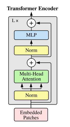
The transformer encoder is a standard transformer encoder architecture as presented in original transformer paper. This encoder takes embedded patches (patch embedding, position embedding and class embedding). The transformer encoder consists of alternating layers of multuheaded self-attention and MLP blocks. Layer Normalization is used before every block and residual connection is used after every block.
Using hybrid architecture
Previously, image patches were used to form input sequence, another approach to form input sequence can be the feature map of a CNN (Convolution Neural Network). Here, the patches extracted from CNN map is used as patch embedding. From the paper:
As an alternative to raw image patches, the input sequence can be formed from feature maps of a CNN. In this hybrid model, the patch embedding projection E (Eq. 1) is applied to patches extracted from a CNN feature map. As a special case, the patches can have spatial size 1x1, which means that the input sequence is obtained by simply flattening the spatial dimensions of the feature map and projecting to the Transformer dimension.