Various self-supervised learning methods have been proposed in recent years for learning image representations. Though a lot of methods have been proposed, the performance of those methods was found less effective in terms of accuracy than those of supervised counterparts. But SimCLR has provided promising results, thus taking self-supervised learning to a new level. It uses a contrastive learning approach. This paper introduces a simple framework to learn representations from unlabeled images based on heavy data augmentation. Before going deep into simCLR and its details, let’s see what contrastive learning is:
Contrastive Learning
Contrastive learning is a framework that learns similarities/dissimilarities from data that are organized into similar/dissimilar parts. It can also be considered as learning by comparing. Contrastive learning learns by comparing among different samples. The samples can be performed between positive pairs of ‘similar’ inputs and negative pairs of ‘dissimilar’ inputs.
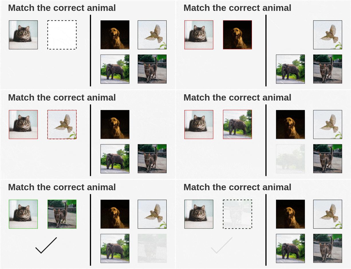
To illustrate this in another way, you’re told to chose a picture that is similar to the picture on the left i.e, cat (on the image below). You look at the picture and find the image from a bunch of images present(on the right side) that is similar to the cat. This way, you contrast between similar and dissimilar objects. The same is the case with contrastive learning. Using this approach we can train a machine learning model to classify between similar and dissimilar objects.

Source: GoogleAI
Contrastive learning approaches only need to define the similarity distribution in order to sample a positive input \(x^{+} \sim\ p^{+}\)
Contrastive learning approaches only need to define the similarity distribution in order to sample a positive input \(x^{+} \sim\ {p^{+}(.|x)}\), and a data distribution for a negative input \(x^{-} \sim\ p^{-}(.|x)\), with respect to an input sample \(x\). The goal of Contrastive learning is: the representation of similar samples should be mapped close together, while that of dissimilar samples should be further away from embedding space.
Source: Contrastive Representation Learning: A Framework and Review
A Simple Framework for Contrastive Learning of Visual Representations - SimCLR
How does simCLR learn representations?
simCLR learns representations by maximizing agreement between differently augmented views of the same data example via a contrastive loss.
Inorder to learn good contrastive representation learning, simCLR consists of four major components
-Data Augmentation module: Data augmentation is more beneficial for unsupervised contrastive learning than supervised learning. The data augmentation module transforms any given data example into two correlated views of the same example. These examples are denoted as \(\\widetilde{x\_i}\) and \(\\widetilde{x\_j}\), considered as positive pair. The authors mainly applied three augmentations sequentially: random cropping followed by resizing to the original size, random color distortions, and random Gaussian blur.
- Encoder: A neural base encoder \(f(.)\) is used that extracts features from augmented data examples. ResNet is used as the architecture to extract those representations. The learned representation is the result of the average pooling layer.
- Projection head: The projection head \(g(.)\) is a MLP with one hidden layer that maps representations from the base encoder network to space where contrastive loss is applied. Here ReLU activation function is used for non-linearity.
- Contrastive loss function: For any given set of \(\\widetilde{x\_k}\) which includes positive example pair \(\\widetilde{x\_i}\) and \(\\widetilde{x\_j}\), contrastive prediction task aims to identify \(\\widetilde{x\_j}\) in {\(\\widetilde{x\_k}\)} (here i and k are not equal) for given \(\\widetilde{x\_i}\)

simCLR Framework Google AI
Working of simCLR algorithm
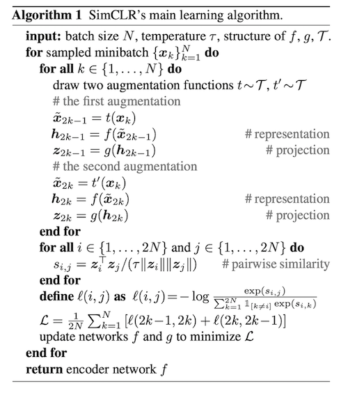
First, we generate a batch of N examples and define contrastive prediction tasks on augmented examples. After applying a series of data augmentation techniques random(crop + resize + color distortion + grayscale) on N examples, 2N data points are generated (since we are generating similar pairs in a batch). Each augmented image is passed in a pair through the base encoder to get a representation from the image. Followed by the base encoder, a projection head is used that maps the base encoder to the representation \(z\_i\) and \(z\_j\) as presented in the paper. For each augmented image, we get embedding vectors for it. These embedding vectors are later subjected for calculating loss.

simCLR algorithm
Calculating loss
After getting the representations of the augmented images, the similarity of those images is calculated using cosine similarity. For two augmented image, \(x\_i\) and \(x\_j\), cosine similarity is calculated on projected representations \(z\_i\) and \(z\_j\).
\(s\_{i,j} = \\frac{z\_i^{T}z\_j}{||z\_i||||z\_j||}\), where
\(T\) denotes a temperature parameter,
\(||z||\) is the norm of the vector
simCLR uses NT-Xent (Normalized temperature-scaled cross entropy loss) for calculating the loss.

Here \(z\_i\) and \(z\_j\) are the output vectors obtained from the projection head
After training simCLR on the contrastive learning task, it can be used for transfer learning. For downstream tasks, representations from encoder are used rather than the representation from projection head. These representations can be used for tasks such as classification, detection.
Results
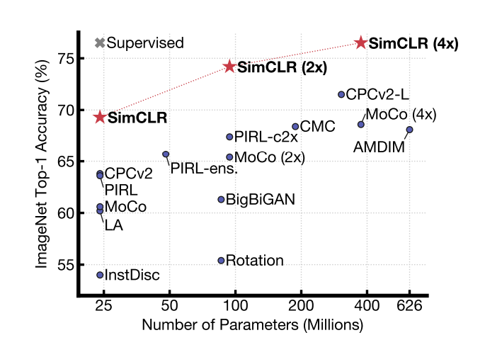
The proposed simCLR outperformed previous self-supervised and semi-supervised methods on ImageNet. A linear classifier trained on self-supervised representations learned by SimCLR achieves 76.5% top-1 accuracy, which is a 7% relative improvement over previous state-of-the-art, matching the performance of a supervised ResNet-50. When fine-tuned on only 1% of the labels, we achieve 85.8% top-5 accuracy, outperforming AlexNet with 100× fewer labels.

ImageNet Top-1 accuracy of linear classifiers trained
on representations learned with different self-supervised methods (pre-trained on ImageNet). Gray cross indicates supervised
ResNet-50. Our method, SimCLR, is shown in bold