In this blog post, I will try to write about the MobileNets and its architecture. MobileNet uses depthwise separable convolutions instead of standard convolution to reduce model size and computation. Hence, it can be used to build light weight deep neural networks for mobile and embedded vision applications.
Topics Covered
- Standard convolutions and depthwise separable convolutions
- MobileNet Architecture
- Width Multiplier to achieve thinner models
- Resolution Multiplier for reduced representation
- Architecture Implementation
Standard convolutions and depthwise separable convolutions
Convolution operation consists of an input image, a kernel or filter that slides through the input image and outputs a feature map. The main aim of convolution operation is to extract features from the input image. As we know, every image can be considered as a matrix of pixel values. Consider an input as 5x5 matrix with values of pixels 0 and 1 as shown below:
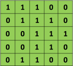
Also, consider another 3x3 matrix as below:

The convolution operation for input size 5x5 with filter of 3x3 is shown below:
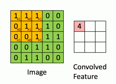
Fig: The Convolution operation. source
We are sliding the 3x3 matrix over 5x5 input matrix and performing element-wise matrix multiplication and adding the multiplication output to get convolved feature. The output obtained from such operation is also called as feature map. The 3x3 matrix that is sliding over the input matrix is known as filter or kernel. More on convolution can be found at this amazing article.
Separable Convolutions
Before knowing what depth-wise separable convolutions do, let’s know about separable convolutions. There are two types of separable convolutions: spatial separable convolutions and depthwise separable convolutions.
Spatial separable convolutions
Spatial Separable convolutions deals with spatial dimension of the image (width and height). It divides a kernel into two smaller kernel. For example, a \(3\*3\) kernel is divided into a \(3\*1\) and a \(1\*3\) kernel.

Here, instead of doing one convolution with 9 multiplicants, we can do two convolutions with 3 multiplications each (i.e., 6 in total) to achieve the same effect. With less multiplications, computational complexity goes down and network is able is run faster.
One of the famous convolution used to detect edges i.e., Sobel kernel can also be separated spatially.

Though, less computation power is achieved using spatial separable convolution, all the kernels cannot be separated into two smaller kernels, which is one of the cons of spatial separable convolution.
Depthwise Separable Convolutions
Depthwise Separable Convolutions is what Mobilenet architecture is based on. Depthwise separable convolution works with kernel that cannot be factored into two smaller kernels. Spatial separable convolutions deals with spatial dimensions but depthwise separable convolutions deals with depth dimension also.
Depthwise separable convolution is a factorized convolution that factorizes standard convolution into a depthwise convolution and a \(1*1\) convolution called pointwise convolution. Depthwise separable convolutions splits kernel into two separate kernels for filtering and combining. Depthwise convolution is used for filterning whereas pointwise convolution is used for combining.
Using depthwise separable convolutions, the total computation required for the operation is the sum of depthwise convolution and pointwise convolution which is:
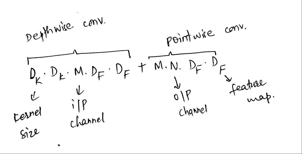
For standard convolution, total computation is:
\(D_K . D_K . M . N . D_F . D_F\), where computational cost depends on number of input channels \(M\), number of output channels \(N\), kernel size \(D_K\) and feature map size \(D_F\).
By expressing convolution as a two steps process of filtering and combining, total reduction in computation is:
\(\frac{D_K . D_K . M . D_F . D_F + M . N . D_F . D_F}{D_K . D_K . M. N. D_F . D_F}\), which is equivalent to \(\frac{1}{N} + \frac{1}{D_k^2}\)
That means when \(D_K * D_K\) is 3*3, computation cost can be reduced to 8 to 9 times.
More on depthwise separable convolutions can be found here.
MobileNet Architecture
- As mentioned above, mobilenet is built on depthwise separable convolutions, except for first layer. First layer is a full convolutional layer.
- All layers are followed by batch normalization and ReLU non-linearity. However, final layer is a fully connected layer without any non-linearity and feeds to the softmax for classification.
- For down sampling, strided convolution is used for both depthwise convolution as well as for first fully convolutional layer.
- The total number of layers for mobilenet is 28 considering depthwise and pointwise convolution as separate layers.
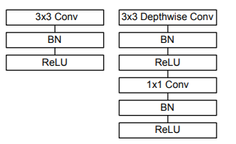
fig. (left) Standard convolution with batchnorm and relu
(right) depthwise and pointwise convolution followed by batchnorm and relu source
MobileNet architecture is shown below:
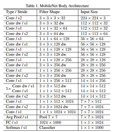
Fig. MobileNet architecture
Width Multiplier to achieve Thinner Models
Though our mobilenet model is smaller and computationally less expensive, sometimes we need our model to be more smaller and less expensive in terms of computation. To construct these models, a separate parameter \(\alpha\) is used called as width multiplier. Width multiplier helps to make network thinner uniformly at each layer. For any given layer and width multiplier \(\alpha\), the number of input channels \(M\) becomes \(\alpha M\) and the number of output channel \(N\) becomes \(\alpha N\). Then, the computational cost for depthwise separable convolution with width multiplier becomes:
\(D_K . D_K . \alpha M . D_F . D_F + \alpha M . \alpha N . D_F . D_F\)
Width multiplier can be applied to any model structure to define a new smaller model with a reasonable accuracy, latency and size trade off. It is used to define a new reduced structure that needs to be trained from scratch. MobileNet paper
Resolution Multiplier for reduced representation
Resolution Multiplier is another parameter for reducing model computational cost. It is represented by \(\rho\). It is applied to the input image and internal representation of every layer is reduced by the same multiplier. The computational cost for depthwise separable convolution with width multiplier becomes:
\(D_K . D_K . \alpha M . \rho D\_F . \rho D_F + \alpha M . \alpha N . \rho D_F . \rho D_F\)
The value of \(\rho\) = 1 is the base mobilenet and \(\rho<1\) is the reduced computational MobileNets.
Architecture Implementation
MobileNet uses depthwise separable convolutions where each layers is followed by BatchNormalization and ReLU non-linearity. MobileNet contains a depthwise and a pointwise convolution layer. The code snippets inspired from MLT.
# First we will build mobilenet block
def mobilenet_block(x, filters, strides):
  x = keras.layers.DepthwiseConv2D(kernel_size=3, strides=strides, padding='same')(x)
  x = keras.layers.BatchNormalization()(x)
  x = keras.layers.ReLU()(x)

  x = keras.layers.Conv2D(filters=filters, kernel_size=1, strides=1, padding='same')(x)
  x = keras.layers.BatchNormalization()(x)
  x = keras.layers.ReLU()(x)
  return x
MobileNet uses input_shape of 224*224*3. First layer of mobilenet is a Convolutional layer with 32 filters, 3*3 kernel and stride of 2. This is followed by BatchNormalization and ReLU non-linearity.
INPUT_SHAPE = 28, 28, 3
input = keras.layers.Input(INPUT_SHAPE)
x = keras.layers.Conv2D(filters=32, kernel_size=3, strides=2, padding='same')(input)
x = keras.layers.BatchNormalization()(x)
x = keras.layers.ReLU()(x)
After first layers, there is a series of mobilenet block with different kernel sizes and filters.
x = mobilenet_block(x, filters=64, strides=1)

x = mobilenet_block(x, filters=128, strides=2)
x = mobilenet_block(x, filters=128, strides=1)

x = mobilenet_block(x, filters=256, strides=2)
x = mobilenet_block(x, filters=256, strides=1)

x = mobilenet_block(x, filters=512, strides=2)
for _ in range(5):
  x = mobilenet_block(x, filters=512, strides=1)
  x = keras.layers.AveragePooling2D(pool_size=7, strides=1)(x)
  output = keras.layers.Dense(1000, activation='softmax')(x)