Have you ever used an app called Prisma that styles your image using popular paintings and turns your photo stunning? If that’s the case then, the app you are using is the result of style transfer; a computer vision technique that combines your images with artistic style.

Introduction

Style transfer is a computer vision technique that takes two images: content image and style image, combines them to form a resulting image that style the image based on style image taking contents from the content image.

Here is how it looks like:

The content image you can see above is Van Gogh’s Starry Night Painting and the style image a image from Tubingen university from Germany. Resultant image is shown on the right side that used content of content image and is styled using style image.

Now let’s get into the working of neural style transfer

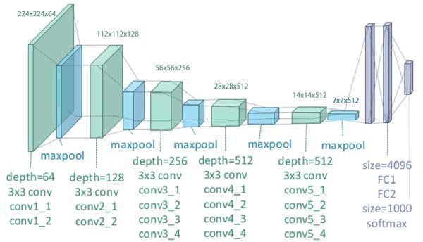
Neural Style Transfer is based on Deep Neural Network that create images of high perpetual quality. It uses neural network to separate and recombine content and style of images that we feed to obtain the desired result. The original paper uses 19 layer VGG network comprising of 16 convolutional layers, 5 max-pooling layers and 3 fully connected layers.

Fig. A 19 layer VGG network source

How exactly do we obtain such images?

Our goal here is to apply style over our content image. We are not training any neural network in this case, rather we start from a blank image and optimize the cost function by changing the pixel values of the image. The cost function contains two losses: Content loss and Style loss.

Considering c as the content image and x as the style transferred image, content loss tends to \(0\) when \(x\) and \(c\) are close to each other and increases when these value gets increased.

Given the original image \(vec{p}\) and generated image \(vec{x}\), we can define the loss generated by the content image as:

Content loss takes content weight which is a scalar that gives weighting for the content loss, content_current that gives features of the current image. content_current is the Pytorch tensor having shape (1, \(C_l\), \(H_l\), \(W_l\)), where
\(C_l\) is the number of channels in layer \(l\), \(H_l\) and \(W_l\) are width and height.

Content loss in python

def content_loss(content_weight, content_current, content_original):
    return torch.sum(content_weight * (content_current-content_original)**2)

After computing content loss, we can compute style loss.
To compute style loss, we need to first compute Gram matrix \(G\). Gram matrix represents the correlation between responses of each filter. Given a feature map \(F^l\) of shape \((C_l, M_l)\), the Gram matrix is given by:

\[G_{ij}^\ell = \sum_k F^{\ell}_{ik} F^{\ell}_{jk}\]

Gram matrix in python:

def gram_matrix(features, normalize=True):
    N, C, H, W = features.size()
    features = features.reshape(N, C,-1)

    gram_matrix = torch.zeros([N,C,C]).to(features.device).to(features.dtype)
    for i in range(N):
      gram_matrix[i,:] = torch.mm( features[i,:], features[i,:].t())
      if (normalize):
        gram_matrix /= float(H*W*C)
      return gram_matrix

Now implementing style loss:

def style_loss(feats, style_layers, style_targets, style_weights):
    loss = 0
    for i, layer in enumerate(style_layers):
      gram_feat = gram_matrix(feats[layer])
      loss += (style_weights[i] * torch.sum((gram_feat-style_targets[i])**2))
    return loss

To increase the smoothness in the image, we can use another term to our loss that penalizes total variation in the pixel values. We can compute the “total variation” as the sum of the squares of differences in the pixel values for all pairs of pixels that are next to each other (horizontally or vertically). Here we sum the total-variation regualarization for each of the 3 input channels (RGB), and weight the total summed loss by the total variation weight, w_t

Total variational loss in python

def tv_loss(img, tv_weight):
  loss = 0
  loss += torch.sum((img[:,:,1:,:]-img[:,:,:-1,:])**2)
  loss += torch.sum((img[:,:,:,1:]-img[:,:,:,:-1])**2)
  loss *= tv_weight
  return los

Combining above snippets together, we can generate resultant image using content and style images. The complete code is available on github. Code is the homework solution for Deep Learning for Computer Vision taught by Justin Johnson.

Neural style transfer and its working

Introduction

Now let’s get into the working of neural style transfer

How exactly do we obtain such images?

Content loss in python

References