“General Adversarial Nets is the most interesting idea in the last 10 years in machine learning”. This was the statement from Yann LeCun regarding GANs when Ian Goodfellow and co-authors introduced it in 2014. After its first introduction, many research papers are published with various architectures and its use cases.
So what are General Adversarial Networks? What are its use cases. In this post I will try to explain about GANs, its underlying math, use cases and GAN implementation in keras.
Introduction
As stated by Ian Goodfellow on his paper, GAN is a framework for estimating generative models via an adversarial process. During this process, two models are trained. One is called generator \(G\) and another model is called as discriminator \(D\). Generator \(G\) generates new examples that are similar to original data. Discriminator model \(D\) classifies whether the data is real or fake. To keep in simple terms, generator is analogous to counterfeiters, whereas discriminator is analogous to police. Counterfeiters tries to produce fake currency and use it, while police try to detect the fake currency. Counterfeiters come up with new ideas and patterns to make the fake money as similar to the original and fool the police. Similarly, police tries to detect the fake money. Similar is the case with GAN. Generative model tries to create fake data samples and fool the discriminator and discriminator classifies whether data is fake or not. This process goes on until data samples generated by generator are indistinguishable from discriminator.
Consider the following notations for different data points and distributions:
Generator’s distribution: \(p_g\)
Data: \(x\)
Input noise variables: \(p_z(z)\)
Then, \(G\) is a generator model represented by multilayer perceptron with parameters \(\theta_g\) (parameters of weights and biases).
Similarly, \(D\) is a discriminator model also represented by multilayer perceptron \(D(x;\theta\_d)\). Then, \(D(x)\) represents a probability that data \(x\) came from original distribution rather than \(p_g\).
A known dataset serves as input for the discriminator. Training involves presenting samples from the training dataset until it achieves acceptable accuracy. Generator however trains based on whether it fools the discriminator. The input to generator is the data samples from latent space ( e.g, multivariate normal distribution). Then, the output generated by the generator is evaluated by the discriminator. Both generator and discriminator model goes through backpropagation to reduce the loss. During this step, generator generates better data samples (say images), whereas discriminator becomes good in classifying fake samples coming from the generator. This way, discriminator \(D\) and generator \(G\) play two-player min-max game.
Training procedure for GANs
- Take a random noise vector \(z\) and feed to the generator \(G\) to produce fake examples \(x^*\). Here label y=0 for \((x, y)\) input-output pair.
- Take fake data \(x^*\) and real data \(x\) and feed to the discriminator model alternatively.
- Since, discriminator \(D\) is a multilayer perceptron, it outputs value between 0 and 1. These values indicates the probability that input is real.
- Both generator and discriminator calculates their respective loss and perform backpropagation to reduce the loss.
- Discriminator tries to maximize the probability of assigning correct labels to both original data and data from random samples.
- Similarly, generator tries to minimize the discriminator’s ability to detect correct and fake samples.
These two networks go on competing with each other until they reach Nash equilibrium. Nash equilibrium is a point in a game where neither player can improve their situation by changing their strategy. More on Nash equilibrium can be found here. The overview of GAN architecture is shown below:

Fig. GAN
The noise vector z is transformed into x* by a generator model which is then fed into discriminator network. Similarly, data from original sample is also fed into discriminator. The discriminator in result outputs a classification values close to 1 for real data x. While for data x*, discriminator tries to output value 0 indicating that x* is fake.
Derivation of Loss function for GANs
Since, GAN is trained in multilayer perception, its loss can be calculated using cross-entropy loss given as:
\(L(y, y\hat{})\) = \([y\log y\hat{} + (1-y) log(1-y\hat{} )]\)
The label for the data coming from \(p_{data}(x)\) is \(y = 1\) and \(y\hat{}\) = \(D(x)\).
So, the cross-entropy equation becomes: \(L(D(x), 1)\) = \(log(D(x))\) ————–(A)
Similarly, for data coming from generator the label is \(y=0\) and \(y\hat{}=D(G(z))\)
In this case, our cross entropy equation becomes: \(L(D(G(z)), 0)\) = \((1-0) log(1-D(G(z))\) = \(log(1-D(G(z))\) ————–(B)
We know that the objective of discriminator is to correctly classify fake versus real data. To achieve this equations (A) and (B) should be maximized.
\(max\) { \(log (D(x))\) + \(log(1-D(G(z)))\)}
The role of generator is to fool discriminator so as to predict fake data as real, i.e., to achieve \(D(G(z)) = 1\) . So, the objective function for generator is given as:
\(min\) {\(log (D(x))\) + \(log(1-D(G(z)))\)}
Note: \(log(D(x))\) has nothing to do with generator objective function. It is kept to provide compact representation of generator and discriminator objective function in our equation.
Combining the objective function of both discriminator and generator, we get following equation:
\(\min\_{G}\) \(\max\_{D}\) {\(log (D(x))\) + \(log(1-D(G(z)))\)}
All the above equations are written with respect to a single instance of data point (x). To consider all the instances of x, we need to take expectation of the whole arguments present in the equation which results in the following equation:

Applications of GANs
- Image-to-Image Translation
- Image-to-Text Translation
- To generate realistic photographs
- Photo Inpainting and many more
Implementation of GAN
Since, GANs consists of two models, generator and discriminator model, we need to build two models. Before building models let’s import libraries. The code snippets for GAN implementation is taken from GANs in Action book.
from keras.datasets import mnist
from keras.layers import Dense, Flatten, Reshape
from keras.layers.advanced_activations import LeakyReLU
from keras.models import Sequential
from keras.optimizers import Adam
Since we will use mnist data to train our discriminator, we need 28*28 image size for our generator for generating new images.
img_rows = 28
img_cols = 28

channels = 1
img_shape = (img_rows, img_cols, channels)

z_dim  = 100
z_dim is the size of noise vector used as input to generator model
Now, we’ll build a generator model
def build_generator(img_shape, z_dim):
  model = Sequential()

  model.add(Dense(128, input_dim=z_dim))
  model.add(LeakyReLU(alpha=0.01))
  model.add(Dense(28*28*1, activation='tanh'))
  model.add(Reshape(img_shape))
  return model
Similarly, building generator model
def build_discriminator(img_shape):
  model = Sequential()
  model.add(Flatten(input_shape=img_shape))
  model.add(Dense(128))
  model.add(LeakyReLU(alpha=0.01))
  model.add(Dense(1, activation='sigmoid'))
  return model
Now, we will build GAN using generator and discriminator build previously. While using combined model to train generator, we keep the parameters of discriminator model fixed. Also, discriminator is trained as an independently compiled model.
def build_gan(generator, discriminator):
  model = Sequential()
  model.add(generator)
  model.add(discriminator)

  return model

discriminator = build_discriminator(img_shape)
discriminator.compile(loss='binary_crossentropy', optimizer=Adam(), metrics=['accuracy'])

generator = build_generator(img_shape, z_dim)
discriminator.trainable = False
gan = build_gan(generator, discriminator)
gan.compile(loss='binary_crossentropy', optimizer=Adam())
Now, that we have build our GAN model, we now train our GAN model. MNIST images is taken as real examples and fake image is generated from noise vector z. These are used to train discriminator network while keeping generator’s parameters constant. Similarly, fake images are generated and we used those images to train generator network by keeping discriminator’s parameter constant.
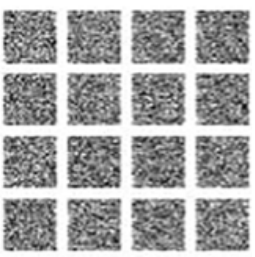
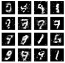
The images produced by generator over the course of training iterations is shown below

During training, random noise is generated and generator gradually learns to imitate the features of training dataset.

This is the output from two layer general adversarial networks. It is gradually imitating the features of MNIST images.
References
- Ian J. Goodfellow et. al. Generative Adversarial Nets.
- https://en.wikipedia.org/wiki/Generative_adversarial_network
- Ahlad Kumar (GAN youtube playlist)