Google proposed a deep Convolution Neural Network named inception that achieved top results for classification and detection in ILSVRC 2014.
The ImageNet Large Scale Visual Recognition Challenge (ILSVRC) evaluates algorithms for object detection and image classification at large scale. One high level motivation is to allow researchers to compare progress in detection across a wider variety of objects – taking advantage of the quite expensive labeling effort. Another motivation is to measure the progress of computer vision for large scale image indexing for retrieval and annotation
“Going deeper with convolutions” is actually inspired by an internet meme: ‘We need to go deeper’

In ILSVRC 2014, GoogLeNet used 12x fewer parameters than AlexNet used 2 years ago in 2012 competition.
Problems Inception v1 is trying to solve
The important parts in the image can have large variation in size. For instance, image of object can be in various positions and some pictures are zoomed in and other may get zoomed out. Because of such variation in images, choosing the right kernel size for performing convolution operation becomes very difficult. We require a larger kernel to extract information of object that is distributed more in the picture and a smaller kernel is preferred to extract information of image that is distributed less in the picture.
One of the major approach to increase the performance of neural networks in by increasing its size. This includes increasing its depth and also its size. Bigger size of neural networks corresponds to larger number of parameters, that makes network more prone to overfitting, especially when labeled training examples are limited.
Another drawback of increased network size is increased use of computational resources. If more convolution layers are chained then there results in more consumption of computation resources. If these added capacity is used ineffectively, then computation resources get wasted.
Solution
To solve these issues, this paper comes up with the solution to form a ‘wider’ network rather than ‘deeper’ which is called as Inception module.

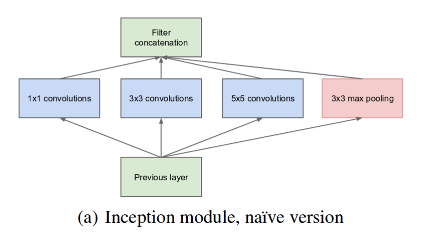
The ‘naive’ inception module performs convolutions on input from previous layer, with 3 different size of kernels or filters specifically 1x1, 3x3, and 5x5. In addition to this, max pooling is also performed. Outputs are then concatenated and sent to the next inception module.
One problem to the ‘naive’ approach is, even having 5x5 convolutions can lead to require large resource in terms of computations. This problem emerges more once pooling is added.
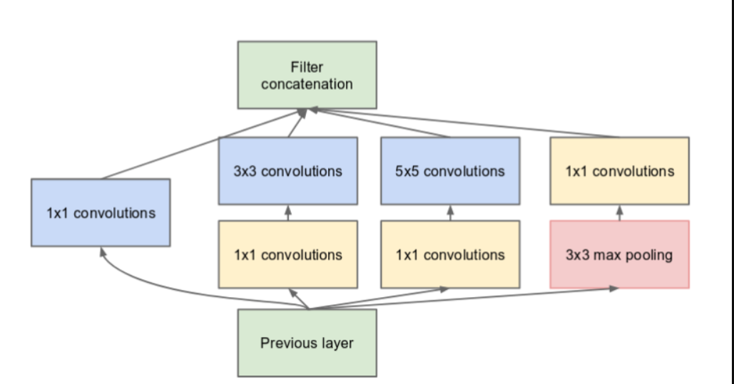
To make our networks inexpensive computationally, authors applied dimensionality reductions by adding 1x1 convolutions before 3x3 and 5x5 convolutions. Let’s see how these affect the number of parameters in the neural network.
Let’s see what 5x5 convolution would be computationally
Computation for above convolution operation is:
(5²)(192)(32)(28²) = 120,422,400 operations
To bring down such a great number of operations, dimensionality reduction can be used. Here, it is done by convolving with 1x1 filters before performing convolution with bigger filters.

5×5 Convolution with Dimensionality Reduction
After dimensionality reduction number of operations for 5x5 convolution becomes:
(1²)(192)(16)(28²) = 2,408,448 operations for the 1 × 1 convolution and,
(5²)(16)(32)(28²) = 10,035,200 operations for the 5 × 5 convolution.
In total there will be 2,408,448 + 10,035,200 = 12,443,648 operations. There is large amount of reduction in computation.
So, after applying dimensionality reduction, our inception module becomes:
GoogLeNet was built using inception module with dimensionality reduction. GoogLeNet consists of 22 layers deep network (27 with pooling layers included). All the convolutions, including the convolutions inside inception module , uses rectified linear activation.

GoogLeNet incarnation of the Inception architecture. Source: Original Paper
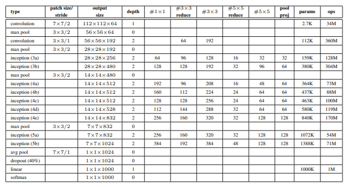
All the convolutions, including those inside the Inception modules, use rectified linear activation. The size of the receptive field in our network is 224x224 taking RGB color channels with mean sub-traction. “#3x3reduce” and “#5x5reduce” stands for the number of 1x1 filters in the reduction layer used before the 3x3 and 5x5 convolutions. One can see the number of 1x1 filters in the pro-jection layer after the built-in max-pooling in the pool proj column. All these reduction/projection layers use rectified linear activation as well
Original Paper
GoogLeNet is 22 layer deep counting only layers with parameters. With such deep network the may arise a problem such as vanishing gradient. To eliminate this, authors introduced auxiliary classifiers that are connected to intermediate layers, and helps the gradient signals to propagate back. These auxiliary classifiers are added on top of the output of Inception (4a) and (4d) modules. The loss from auxiliary classifiers are added during training and discarded during inference.
The exact structure of the extra network on the side, including the auxiliary classifier, is as follows:
- An average pooling layer with 5x5 filter size and stride 3, resulting in an 4x4 512 output for the (4a), and 4x4 528 for the (4d) stage.
- A 1x1 convolution with 128 filters for dimension reduction and rectified linear activation.
- A fully connected layer with 1024 units and rectified linear activation.
- A dropout layer with 70% ratio of dropped outputs
- A linear layer with softmax loss as the classifier (predicting the same 1000 classes as the main classifier, but removed at inference time).
The systematic view of GoogLeNet architecture is shown below:

GoogLeNet architecture
GoogLeNet consists of a total of 9 inception modules namely 3a, 3b, 4a, 4b, 4c, 4d , 4e, 5a and 5b.
GoogLeNet implementation
Having known about inception module and its inclusion in GoogLeNet architecture, we now implement GoogLeNet in tensorflow. This implementation of GoogLeNet is inspired from analytics vidya article on inception net.
Importing the required libraries:
from tensorflow.keras.layers import Layer
import tensorflow.keras.backend as K
import tensorflow as tf
from tensorflow.keras.datasets import cifar10
from tensorflow.keras.models import Model
from tensorflow.keras.layers import Conv2D, MaxPool2D, Dropout, Dense, Input, concatenate, GlobalAveragePooling2D, AveragePooling2D, Flatten
import cv2
import numpy as np
from keras.utils import np_utils
import math
from tensorflow.keras.optimizers import SGD
from tensorflow.keras.callbacks import LearningRateScheduler
Next we are using cifar10 dataset as our data.
num_classes = 10
def load_cifar_data(img_rows, img_cols):
  #Loading training and validation datasets
  (X_train, Y_train), (X_valid, Y_valid) = cifar10.load_data()
  #Resizing images
  X_train = np.array([cv2.resize(img, (img_rows, img_cols)) for img in X_train[:,:,:,:]])
  X_valid = np.array([cv2.resize(img, (img_rows, img_cols)) for img in X_valid[:,:,:,:]])
  #Transform targets to keras compatible format
  Y_train = np_utils.to_categorical(Y_train, num_classes)
  Y_valid = np_utils.to_categorical(Y_valid, num_classes)
  X_train = X_train.astype('float32')
  X_valid = X_valid.astype('float32')
  #Preprocessing data
  X_train = X_train / 255.0
  Y_train = X_valid / 255.0
  return X_train, Y_train, X_valid, Y_valid

X_train, Y_trian, X_test, y_test = load_cifar_data(224,224)
Next comes our inception module
Inception module contains 1x1 convolutions before 3x3 and 5x5 convolution operations. It takes different number of filters for different convolution operations and concatenate these operations to take into next layer.
def inception_module(x, filters_1x1, filters_3x3_reduce, filters_3x3, filters_5x5_reduce, filters_5x5, filters_pool_proj, name=None):
  conv_1x1 = Conv2D(filters_1x1, (1,1), activation='relu', kernel_initializer=kernel_init, bias_initializer=bias_init)(x)
  conv_3x3 = Conv2D(filters_3x3_reduce, (1,1), padding='same', activation='relu', kernel_initializer=kernel_init, bias_initializer=bias_init)(x)
  conv_3x3 = Conv2D(filters_3x3, (3,3), padding='same', activation='relu', kernel_initializer=kernel_init, bias_initializer=bias_init)(conv_3x3)
  conv_5x5 = Conv2D(filters_5x5_reduce, (1,1), padding='same', activation='relu', kernel_initializer=kernel_init, bias_initializer=bias_init)(x)
  conv_5x5 = Conv2D(filters_5x5, (3,3), padding='same', activation='relu', kernel_initializer=kernel_init, bias_initializer=bias_init)(conv_5x5)
  pool_proj = MaxPool2D((3,3), strides=(1,1), padding='same')(x)
  pool_proj = Conv2D(filters_pool_proj, (1, 1), padding='same', activation='relu', kernel_initializer=kernel_init, bias_initializer=bias_init)(pool_proj)
  output = concatenate([conv_1x1, conv_3x3, conv_5x5, pool_proj], axis=3, name=name)
  return output

import tensorflow
kernel_init = tensorflow.keras.initializers.GlorotUniform()
bias_init = tensorflow.initializers.Constant(value=0.2)

input_layer = Input(shape=(224, 224, 3))
x = Conv2D(64, (7,7), padding='same', strides=(2, 2), activation='relu', name='conv_1_7x7/2', kernel_initializer=kernel_init, bias_initializer=bias_init)(input_layer)
x = MaxPool2D((3,3), padding='same', strides=(2,2), name='max_pool_1_3x3/2')(x)
x = Conv2D(64, (1,1), padding='same', strides=(1, 1), activation='relu', name='conv_2a_3x3/1', kernel_initializer=kernel_init, bias_initializer=bias_init)(x)
x = Conv2D(192, (3,3), padding='same', strides=(1, 1), activation='relu', name='conv_2b_3x3/1', kernel_initializer=kernel_init, bias_initializer=bias_init)(x)
x = MaxPool2D((3,3), padding='same', strides=(2, 2), name='max_pool_2_3x3/2')(x)
x = inception_module(x,
                     filters_1x1=64,
                     filters_3x3_reduce=96,
                     filters_3x3=128,
                     filters_5x5_reduce=16,
                     filters_5x5=32,
                     filters_pool_proj=32,
                     name='inception_3a')
x = inception_module(x,
                     filters_1x1=128,
                     filters_3x3_reduce=128,
                     filters_3x3=192,
                     filters_5x5_reduce=32,
                     filters_5x5=96,
                     filters_pool_proj=64,
                     name='inception_3b')
x = MaxPool2D((3,3), strides=(2, 2), padding='same', name='max_pool_3_3x3/2')(x)
x = inception_module(x,
                     filters_1x1=192,
                     filters_3x3_reduce=96,
                     filters_3x3=208,
                     filters_5x5_reduce=16,
                     filters_5x5=48,
                     filters_pool_proj=64,
                     name='inception_4a')
x1 = AveragePooling2D((5,5), strides=3)(x)
x1 = Conv2D(128, (1,1), padding='same', activation='relu')(x1)
x1 = Flatten()(x1)
x1 = Dense(1024, activation='relu')(x1)
x1 = Dropout(0.4)(x1)
x1 = Dense(10, activation='softmax', name='auxiliary_output_1')(x1)
x = inception_module(x,
                     filters_1x1=160,
                     filters_3x3_reduce=112,
                     filters_3x3=224,
                     filters_5x5_reduce=24,
                     filters_5x5=64,
                     filters_pool_proj=64,
                     name='inception_4b')
x = inception_module(x,
                     filters_1x1=128,
                     filters_3x3_reduce=128,
                     filters_3x3=256,
                     filters_5x5_reduce=24,
                     filters_5x5=64,
                     filters_pool_proj=64,
                     name='inception_4c')
x = inception_module(x,
                     filters_1x1=112,
                     filters_3x3_reduce=144,
                     filters_3x3=288,
                     filters_5x5_reduce=32,
                     filters_5x5=64,
                     filters_pool_proj=64,
                     name='inception_4d')
x2 = AveragePooling2D((5,5), strides=3)(x)
x2 = Conv2D(128, (1,1), padding='same', activation='relu')(x2)
x2 = Flatten()(x2)
x2 = Dense(1024, activation='relu')(x2)
x2 = Dropout(0.4)(x2)
x2 = Dense(10, activation='softmax', name='auxiliary_output_2')(x2)
x = inception_module(x,
                     filters_1x1=256,
                     filters_3x3_reduce=160,
                     filters_3x3=320,
                     filters_5x5_reduce=32,
                     filters_5x5=128,
                     filters_pool_proj=128,
                     name='inception_4e')
x = MaxPool2D((3,3), strides=(2,2), padding='same', name='max_pool_4_3x3/2')
x = inception_module(x,
                     filters_1x1=256,
                     filters_3x3_reduce=160,
                     filters_3x3=320,
                     filters_5x5_reduce=32,
                     filters_5x5=128,
                     filters_pool_proj=128,
                     name='inception_5a')
x = inception_module(x,
                     filters_1x1=384,
                     filters_3x3_reduce=192,
                     filters_3x3=384,
                     filters_5x5_reduce=48,
                     filters_5x5=128,
                     filters_pool_proj=128,
                     name='inception_5b')
x = GlobalAveragePooling2D(name='avg_pool_5_3x3/1')(x)
x = Dropout(0.4)(x)
x = Dense(10, activation='softmax', name='output')(x)

model = Model(input_layer, [x, x1, x2], name='inception_v1')
Getting the summary of the model
model.summary()epochs = 25
initial_lrate = 0.01
def decay(epoch, steps=100):
initial_lrate = 0.01
drop = 0.96
epochs_drop = 8
lrate = initial_lrate * math.pow(drop, math.floor((1+epoch)/epochs_drop))
return lrate
sgd = SGD(lr=initial_lrate, momentum=0.9, nesterov=False)
lr_sc = LearningRateScheduler(decay, verbose=1)
model.compile(loss=['categorical_crossentropy', 'categorical_crossentropy', 'categorical_crossentropy'], loss_weights=[1, 0.3, 0.3], optimizer=sgd, metrics=['accuracy'])Using our model to fit the training data
history = model.fit(X_train, [y_train, y_train, y_train], validation_data=(X_test, [y_test, y_test, y_test]), epochs=epochs, batch_size=256, callbacks=[lr_sc])References