VGGNet is a Convolutional Neural Network architecture proposed by Karen Simonyan and Andrew Zisserman of University of Oxford in 2014. This paper mailny focuses in the effect of the convolutional neural network depth on its accuracy. You can find the original paper of VGGNet which is titled as Very Deep Convolutional Networks for Large Scale Image Recognition.
Architecture
The input to VGG based convNet is a 224*224 RGB image. Preprocessing layer takes the RGB image with pixel values in the range of 0 - 255 and subtracts the mean image values which is calculated over the entire ImageNet training set.

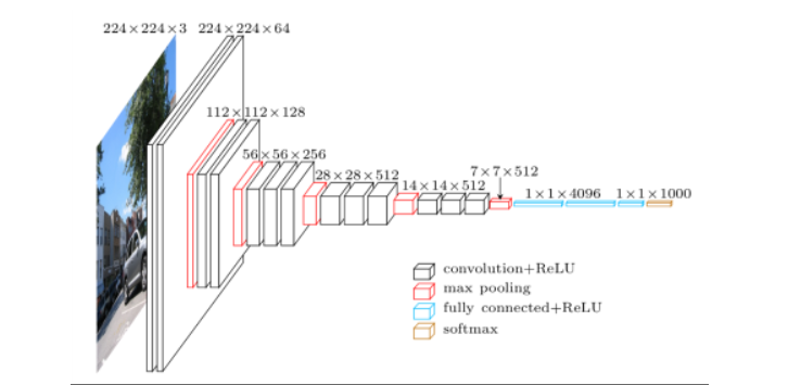
Fig. A visualization of the VGG architecture (source)
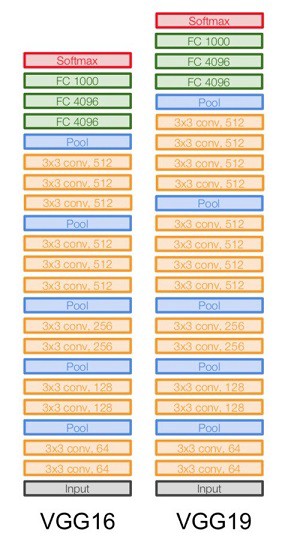
The input images after preprocessing are passed through these weight layers. The training images are passed through a stack of convolution layers. There are total of 13 convolutional layers and 3 fully connected layers in VGG16 architecture. VGG has smaller filters (3*3) with more depth instead of having large filters. It has ended up having the same effective receptive field as if you only have one 7 x 7 convolutional layers.
Another variation of VGGNet has 19 weight layers consisting of 16 convolutional layers with 3 fully connected layers and same 5 pooling layers. In both variation of VGGNet there consists of two Fully Connected layers with 4096 channels each which is followed by another fully connected layer with 1000 channels to predict 1000 labels. Last fully connected layer uses softmax layer for classification purpose.

VGG 16 and VGG 19 Layers ( source)
Architecture walkthrough:
- The first two layers are convolutional layers with 3x3 filters, and first two layers use 64 filters that results in 224x224x64 volume as same convolutions are used. The filters are always 3x3 with stride of 1
- After this, pooling layer was used with max-pool of 2x2 size and stride 2 which reduces height and width of a volume from 224x224x64 to 112x112x64.
- This is followed by 2 more convolution layers with 128 filters. This results in the new dimension of 112x112x128.
- After pooling layer is used, volume is reduced to 56x56x128.
- Two more convolution layers are added with 256 filters each followed by down sampling layer that reduces the size to 28x28x256.
- Two more stack each with 3 convolution layer is separated by a max-pool layer.
- After the final pooling layer, 7x7x512 volume is flattened into Fully Connected (FC) layer with 4096 channels and softmax output of 1000 classes.
Implementation
Now let’s go ahead and see how we can implement this architecture using tensorflow. This implementation is inspired from Machine Learning Tokyo’s CNN architectures.
Importing libraries
Starting the convolution blocks with the input layer
input = Input(shape=(224,224,3))1st block consists of 2 convolution layer each with 64 filters of 3*3 and followed by a max-pool layer with stride 2 and pool-size of 2. All hidden layer uses ReLU for non-linearity.
x = Conv2D(filters=64, kernel_size=3, padding='same', activation='relu')(input)
x = Conv2D(filters=64, kernel_size=3, padding='same', activation='relu')(x)
x = MaxPool2D(pool_size=2, strides=2, padding='same')(x)
2nd block also consists of 2 convolution layer each with 128 filters of 3*3 and followed by a max-pool layer with stride 2 and pool-size of 2.
x = Conv2D(filters=128, kernel_size=3, padding='same', activation='relu')(x)
x = Conv2D(filters=128, kernel_size=3, padding='same', activation='relu')(x)
x = MaxPool2D(pool_size=2, strides=2, padding='same')(x)
3rd block consists of 3 convolution layer each with 256 filters of 3*3 and followed by a max-pool layer with stride 2 and pool-size of 2.
x = Conv2D(filters=256, kernel_size=3, padding='same', activation='relu')(x)
x = Conv2D(filters=256, kernel_size=3, padding='same', activation='relu')(x)
x = Conv2D(filters=256, kernel_size=3, padding='same', activation='relu')(x)
x = MaxPool2D(pool_size=2, strides=2, padding='same')(x)
4th and 5th block consists of 3 convolutional layers with 512 filters each. In between these blocks, a max-pool layer is used with stride of 2 and pool-size of 2.
x = Conv2D(filters=512, kernel_size=3, padding='same', activation='relu')(x)
x = Conv2D(filters=512, kernel_size=3, padding='same', activation='relu')(x)
x = Conv2D(filters=512, kernel_size=3, padding='same', activation='relu')(x)
x = MaxPool2D(pool_size=2, strides=2, padding='same')(x)
x = Conv2D(filters=512, kernel_size=3, padding='same', activation='relu')(x)
x = Conv2D(filters=512, kernel_size=3, padding='same', activation='relu')(x)
x = Conv2D(filters=512, kernel_size=3, padding='same', activation='relu')(x)
x = MaxPool2D(pool_size=2, strides=2, padding='same')(x)
The output from 5th convolution block is Flattened which gives 4096 units. This fully connected layer is connected to another FC layer having same number of units. The final fully connected layer contains 1000 units and softmax activation which is used for classification of 1000 classes
#Dense Layers
x = Flatten(x)
x = Dense(units=4096, activation='relu')(x)
x = Dense(units=4096, activation='relu')(x)
output = Dense(units=1000, activation='softmax')(x)
from tensorflow.keras import Model
model = Model(inputs=input, outputs=output)